大数据实战 Python可视化 Matplotlib可视化
本文是关于大数据通过Python的Matplotlib实现数据可视化。
一、实验环境:
- 虚拟机数量:1
- 系统版本:Centos 7.5
- Anaconda版本:4.4.0
二、实验内容:
- 通过创建Kafka topic,使用Kafka Producer产生消息,然后通过编写spark
Streaming程序处理这些消息。 - 主要步骤:
- Matplotlib的介绍
- 基本绘图函数
- 图表的修饰项介绍
- 子图绘制
- 图像的保存
三、实验步骤:
3.1Matplotlib的介绍:
在Python中,主要运用matplotlib库进行数据可视化。matplotlib是Python最著名的绘图库,它提供了一整套和matlab相似的命令API,十分适合交互式地进行制图。而且也可以方便地将它作为绘图控件,嵌入GUI应用程序中。
3.2基本绘图函数:
matplotlib的pyplot子库提供了和matlab类似的绘图API,方便用户快速绘制2D图表。pyplot模块中常见的用来绘制图形的主要有以下几种函数:
3.2.1plot:常用于绘制线型图,该方法具有可变长参数,参数color指定颜色,参数linestyle设置线的样式、参数marker设置标记类型,结果返回一个lines.Line2D对象的列表,lines.Line2D对象的属性可通过plot的关键字参数设置。
3.2.2scatter: 用于绘制散点图;
3.2.3hist:用于绘制直方图,其参数中较为重要的是bins,该参数指定bin(箱子)的个数,即柱状图中柱子的总数,该值默认为10;
3.2.4show: 显示图像。
3.3图表的修饰项介绍:
对于大多数的图表装饰项,其主要实现方式主要有使用过程型的pyplot接口和面向对象的原生matplotlib API两种,分别对应的是函数编程和对象编程两种思想。
3.3.1title:设置或者获取图表标题;
3.3.2xlim:设置或者获取X轴范围;
3.3.3xlabel:设置或者获取X轴标签;
3.3.4**xticks(<刻度>,<标签>)**:设置或者获取X轴刻度和刻度标签;
3.3.5**text(x,y,z)**:将文本z绘制在图表的指定坐标(x,y)
3.3.6legend:自动创建图例,可以通过设置loc参数指定图例的位置。需要事先在添加图像时设置label参数。
3.3.7**twinx(ax)**:返回一个与子图对象ax的x轴一致y轴在右侧的子图对象ax2,用于绘制双轴图表。使用实例方法的形式为ax2=ax.twinx()。
3.3.8除了上面特别说明的,其它方法各自对应子图对象的的两个实例方法,以xlim为例,就是Axes.get_xlim和Axes.set_xlim。
3.4子图绘制:
简单类型的Artists为标准的绘图元件,例如Line2D、Rectangle、Text、AxesImage等等。而容器类型则可以包含许多简单类型的Artists,使它们组织成一个整体,例如Axis、Axes、Figure等。
3.4.1figure:用来创建一个绘图对象,通常也可以不创建绘图对象而调用plot之类的函数直接绘图,matplotlib会自动创建一个绘图对象。通过figsize参数可以指定绘图对象的宽度和高度。如果需要同时绘制多幅图表的话,可以是给figure传递一个整数参数指定图表的序号,如果所指定序号的绘图对象已经存在的话,将不创建新的对象,而只是让它成为当前绘图对象;
3.4.2subplot:创建一个新的Figure,并返回一个含有已创建的subplot对象的NumPy数组。该方法的调用形式为:subplot(numRows,numCols, plotNum),将整个绘图区域等分为numRows行、numCols列个子区域,然后按照从左到右,从上到下的顺序对每个子区域进行编号,左上的子区域的编号为1。如果numRows,numCols和plotNum的值都小于10,可以把它们缩写为一个整数,例如 subplot(321)和subplot(3,2,1)是相同的;对于绘图对象有add_subplot方法用于添加subplot对象;
3.4.3subplots:创建一个包含多个子图的Figure,返回Figure和一个或多个ax(子图)对象,可以通过设置sharex/sharey参数指定共享x轴/y轴;
3.4.4axes:同样往图表添加子图,不同之处在于子图可以设定在绘图区域的任意位置,axes的参数是一个形如[left,bottom, width,height]的列表,这些数值分别指定所创建的Axes对象相对于绘图对象的位置和大小,取值范围都在0到1之间。对于绘图对象有add_axes方法用于添加subplot对象。
3.5图像的保存:
利用plt.savefig可以将当前图表保存到文件,该方法相当于Figure对象的实例方法savefig。具体参数如下:
3.5.1 fname:含有文件路径的字符串或Python的文件型对象;
3.5.2 dpi:图像分辨率(每英寸点数),默认为100;
3.5.3 facecolor,edgecolor,图像的背景色,默认为”w”,即白色;
3.5.4 format:显式设置文件格式(”png”、”pdf”、”svg”等);
3.5.5 bbox_inches:图表需要保存的部分。
3.6Matplotlib 绘图示例
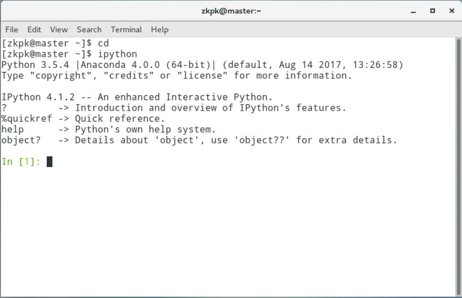
3.6.1执行如下命令打开编程环境
1 | cd |
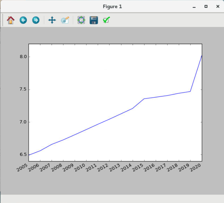
3.6.2绘制世界人口与年份的关系图:
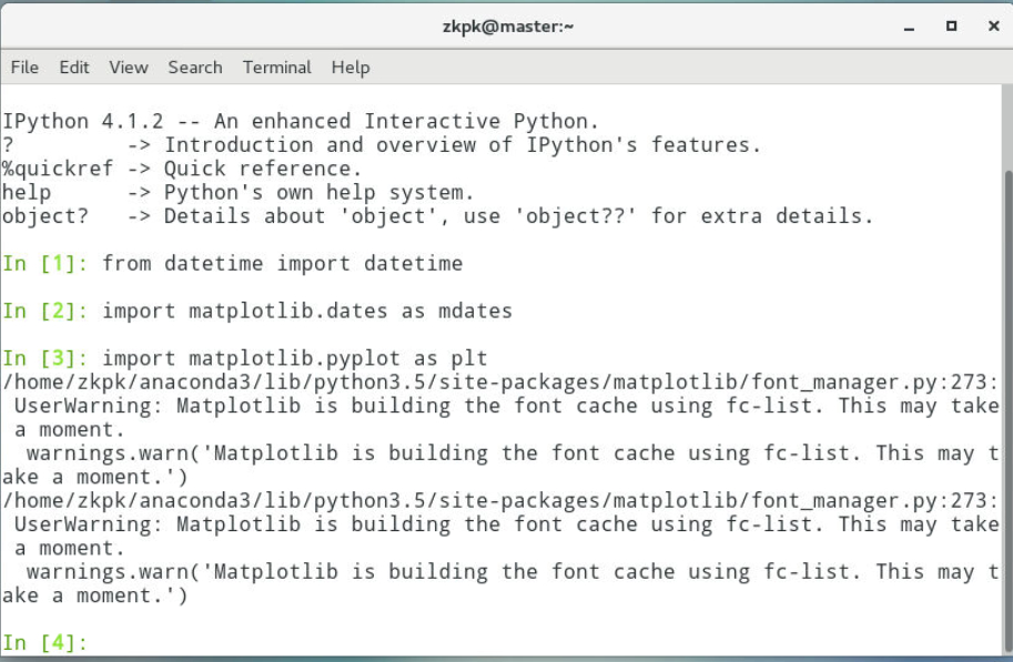
3.6.2.1导入实验所需的库
1 | from datetime import datetime |
3.6.2.2year 和pop为年份和对应的全世界人口数辆(单位10亿)
1 | yearInt = [2005, 2006, 2007, 2008, 2009, 2010, 2011, 2012, 2013, 2014, 2015, 2016, 2017, 2018, 2019, 2020] |
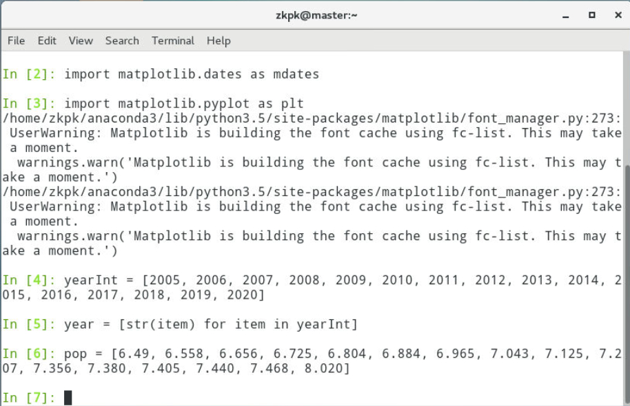
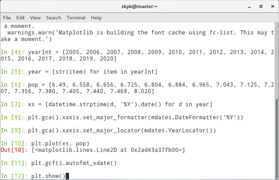
3.6.2.3绘图
1 | xs = [datetime.strptime(d, '%Y').date() for d in year] # 将year中的每个如'2005'的字符串转换成只包含年的日期 |
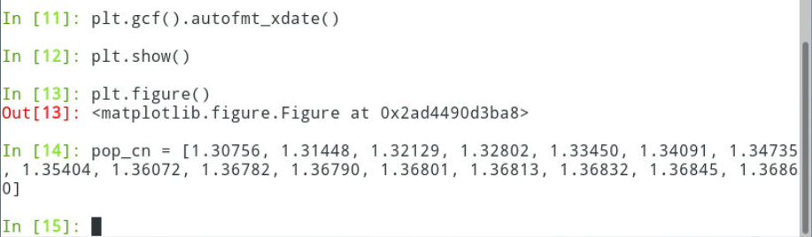
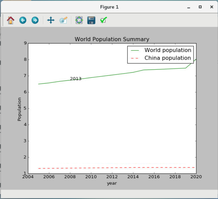
3.7在上一幅图表中添加另一条关于中国人品与年份关系的线,并对新图添加对应的修饰项
3.7.1添加中国人口数量关系
1 | plt.figure() |
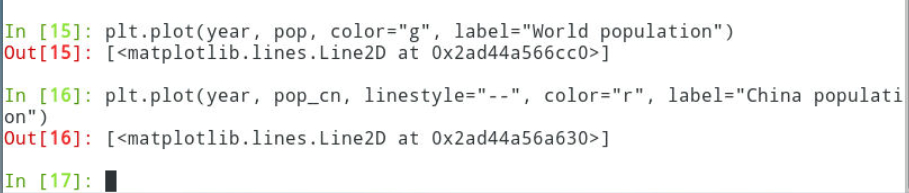
3.7.2绘制人口数量和年份关系;year与pop仍然用之前的数据
1 | plt.plot(year, pop, color="g", label="World population") |
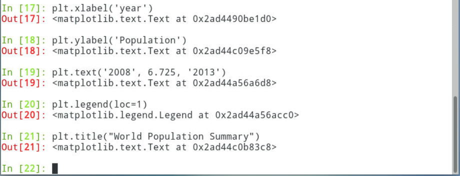
3.7.3添加修饰项
3.7.3.1添加x,y轴标签
3.7.3.2添加注解。注解点为(2008, 6.725),内容为年(2013)
3.7.3.3添加图例,loc=1,表示图例出现在恰当的位置
3.7.3.4添加title
1 | plt.xlabel('year') |
3.7.4显示图片
1 | plt.show() |
3.8子图的绘制:
利用plt.subplots函数创建包含多个子图的绘图对象,还可以设置子图个数。
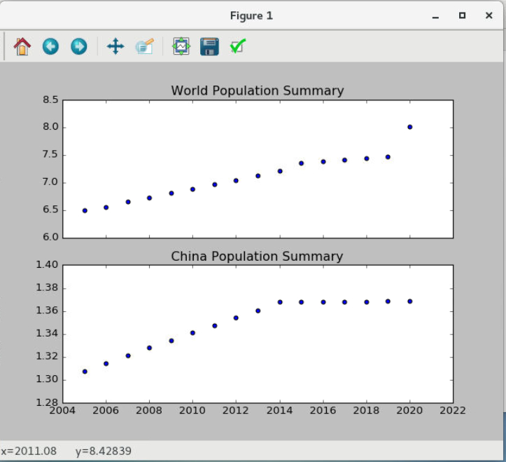
3.8.1绘制x轴共享子图,
3.8.1.1子图个数设置为2,并且共享x轴
1 | f, (ax1, ax2) = plt.subplots(2, sharex=True) # f是Figure对象;ax1,ax2分别是Axes |
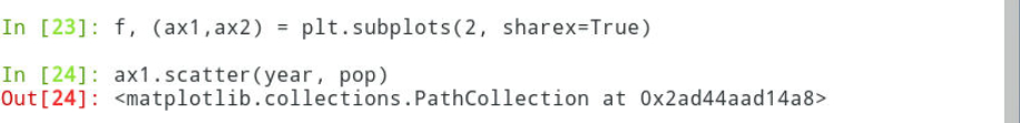
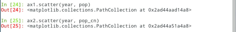
3.8.1.2使用散点图绘制
1 | ax1.scatter(year, pop) # 绘制散点图 |
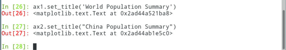
3.8.1.3添加修饰项:标题,
1 | ax1.set_title('World Population Summary') # 设置标题 |
3.8.1.4显示图像
1 | plt.show() |
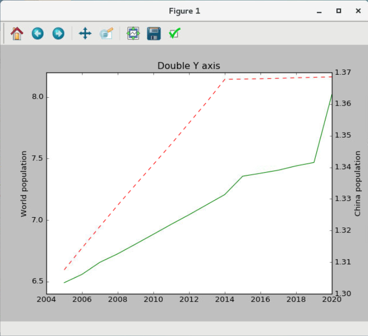
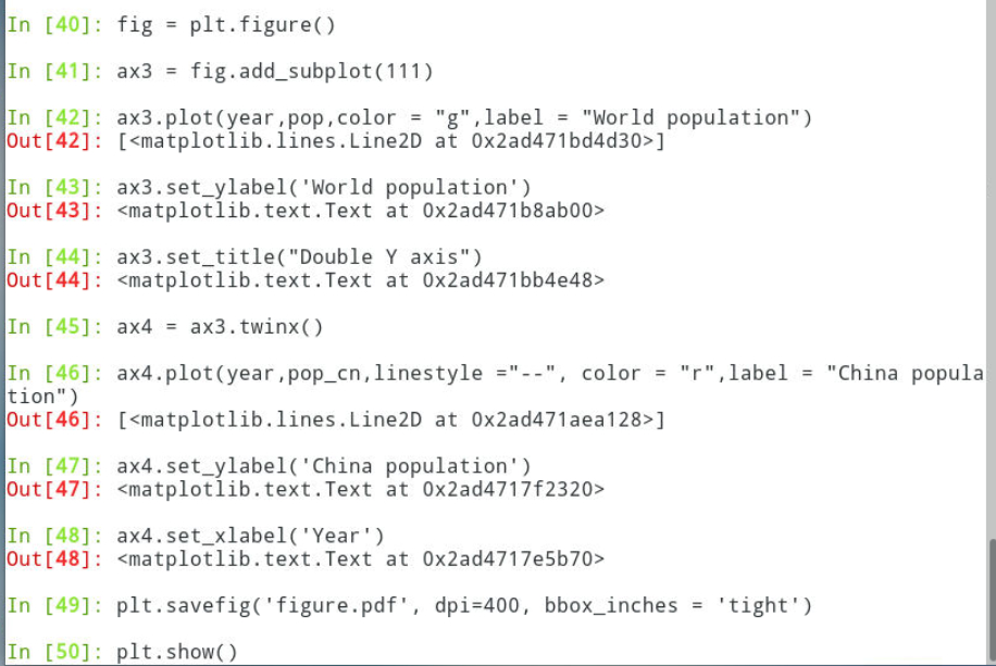
3.8.2绘制双y轴子图,共享x轴。
3.8.2.1创建绘图对象fig
1 | fig = plt.figure() |

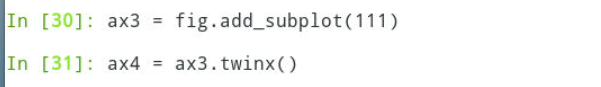
3.8.2.2使用fig.add_subplot函数为绘图对象fig添加两个子图,ax4通过使用ax3的twinx方法创建,且与ax3共享x中,放置在y轴右侧
1 | ax3 = fig.add_subplot(111) # 参数是1个3位的整数或3个分隔的整数,描述子图的位置,分别是nrows,ncols,index |
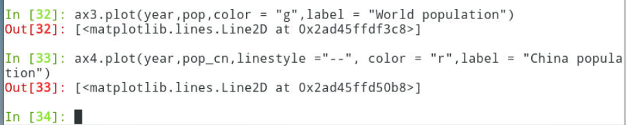
3.8.2.3绘制子图ax3, ax4
1 | ax3.plot(year, pop, color="g", label="World population") |
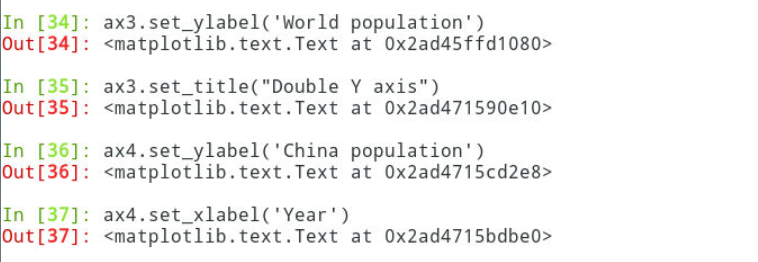
3.8.2.4添加修饰项:添加x,y轴标签、 标题
1 | ax3.set_ylabel('World population') |
3.8.2.5显示图像
1 | plt.show() |
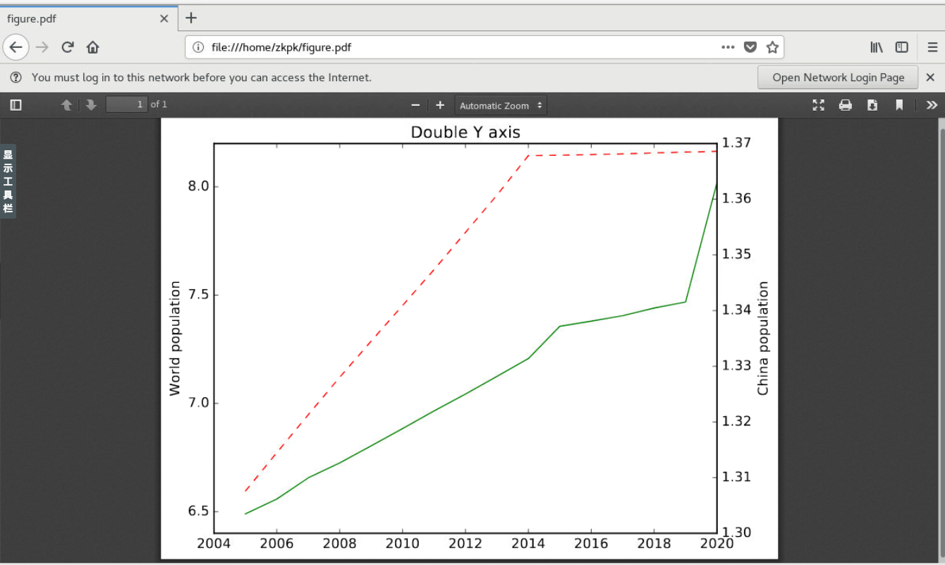
3.9图像的保存:
3.9.1代码使用双y轴的代码,代码末尾show()方法改成保存方法即可
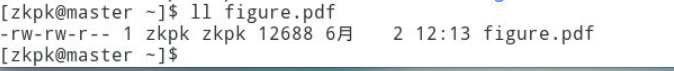
3.9.2使用plt.savfig()函数保存图像
3.9.2.1制定保存的名称,格式,像素,以及是否修渐空白区域。
1 | fig = plt.figure() |
3.9.2.2点击关闭弹出的效果图
3.9.2.3查看保存的文件:打开火狐浏览器,地址栏键入如下内容(生成图片的绝对路径)
四、附录
所有的代码汇总plt.py
点击查看代码
1 | from datetime import datetime |


本文为博主「Sekiro」的原创文章
内容遵循 署名-非商业性使用-相同方式共享 4.0 国际 (CC BY-NC-SA 4.0) 协议